Quartic Hamiltonian

This Hamiltonian models a chemical reaction where the _molecule_ reacts by crossing the barrier separating the double-well (two molecular configurations which are denoted by the bottom of the well) potential and is coupled with the _solvent_ represented by the harmonic oscillator.

\[\begin{equation} \mathcal{H}(x,y,p_x,p_y) = T(p_x, p_y) + V(x, y) = \frac{p_x^2}{2m_A} + \frac{p_y^2}{2m_B} + V(x, y) \end{equation}\]

where the potential energy function \(V_(x,y)\) is

\[\begin{align} V(x,y) = - \alpha \frac{x^2}{2} + \beta \frac{x^4}{4} + \frac{\omega}{2}y^2 + \frac{\epsilon}{2}(x - y)^2 \end{align}\]

The parameters in the model are \(m_A, m_B\) which represent mass of the molecular configurations A and B, while \(\alpha, \beta\) denote features of the potential energy surface geometry, \(\omega, \epsilon\) denote the frequency of the harmonic bath mode, and coupling strength.

Coupled quartic Hamiltonian

We describe the coupled case (\(\epsilon \neq 0.0\)) to illustrate how to set up a script for computing the unstable periodic orbit using the different methods.

The expected result of the computation using differential correction method is the figure below.

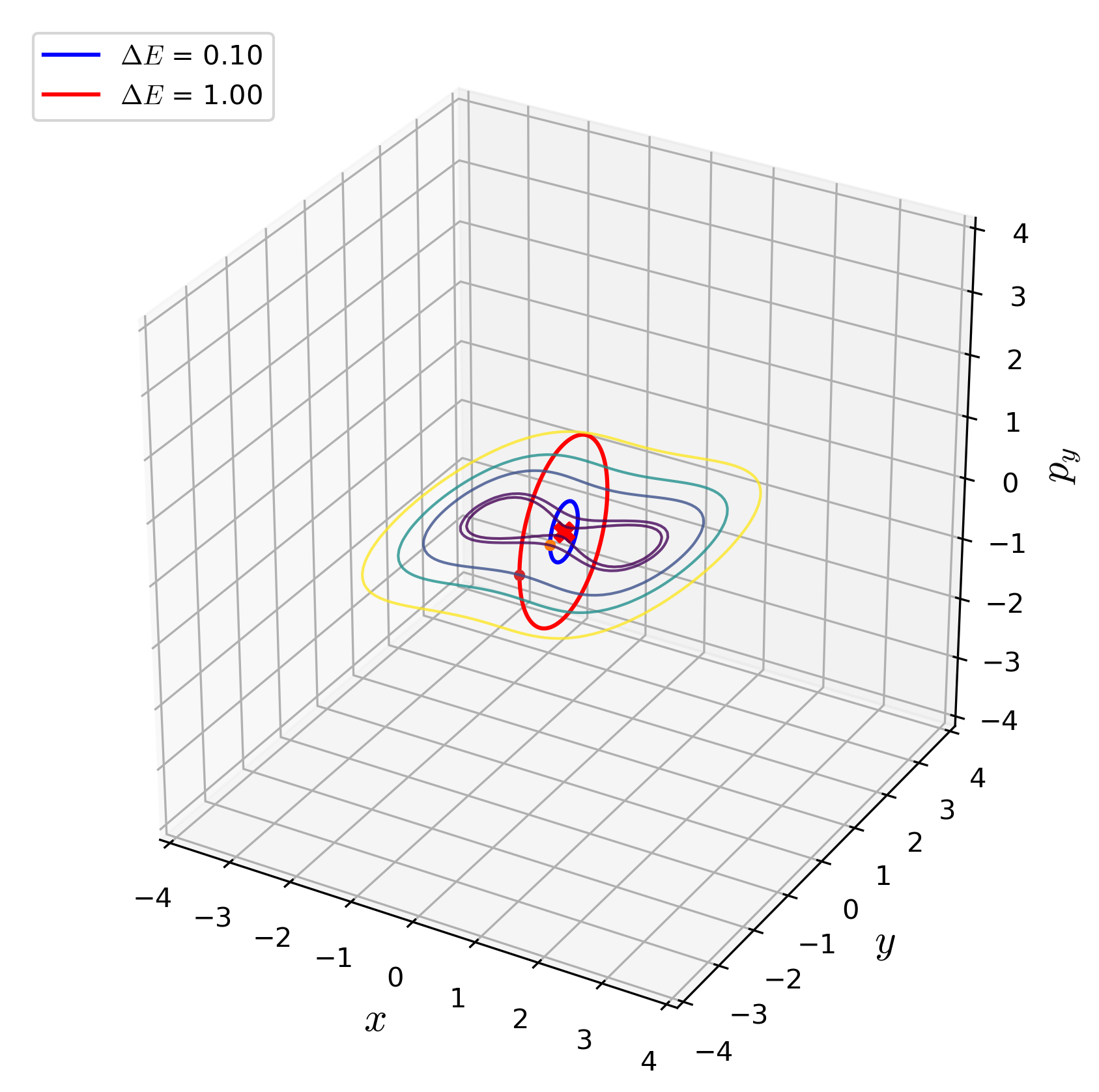
Figure showing the unstable periodic orbits in the bottleneck of the two degrees of freedom coupled quartic Hamiltonian. The unstable periodic orbits at two values of the total energy are shown in red and blue, and the equipotential contours are projected on the \(x-y\) plane (\(p_y = 0\)).

The functions below implement the expressions for this specific Hamiltonian and that are sent as parameters to the functions for a method described in Available methods.

coupled_quartic_hamiltonian.configdiff_coupled(guess1, guess2, ham2dof_model, half_period_model, n_turn, parameters)

Returns the difference of x(or y) coordinates of the guess initial condition and the ith turning point

Used by turning point based on configuration difference method and passed as an argument by the user. Depending on the orientation of a system’s bottleneck in the potential energy surface, this function should return either difference in x coordinates or difference in y coordinates is returned as the result.

Parameters:

• guess1 (float (list of size 4)) – initial condition # 1
• guess2 (float (list of size 4)) – initial condition # 2
• ham2dof_model (function name) – function that returns the Hamiltonian vector field
• half_period_model (function name) – function to catch the half period event during integration
• n_turn (int) – index of the number of turn as a trajectory comes close to an equipotential contour
• parameters (float (list)) – model parameters

Returns:

(x_diff1, x_diff2) or (y_diff1, y_diff2) – difference in the configuration space coordinates, either x or y depending on the orientation of the bottleneck.

Return type:

float (list of size 2)

coupled_quartic_hamiltonian.conv_coord_coupled(x1, y1, dxdot1, dydot1)

Returns the variable we want to keep fixed during differential correction.

dxdot1 -> fix x, dydot1 -> fix y.

Parameters:

• x1 (float) – value of phase space coordinate, x
• y1 (float) – value of phase space coordinate, y
• dxdot1 (float) – value of phase space coordinate, dxdot
• dydot1 (float) – value of phase space coordinate, dydot

Returns:

Return type:

value of one of the phase space coordinates

coupled_quartic_hamiltonian.diffcorr_acc_corr_coupled(coords, phi_t1, x0, parameters)

Returns the updated guess for the initial condition after applying small correction based on the leading order terms.

Correcting x or y coordinate of the guess depends on the system and needs to be chosen by inspecting the geometry of the bottleneck in the potential energy surface.

Parameters:

• coords (float (list of size 4)) – phase space coordinates in the order of position and momentum
• phi_t1 (2d numpy array) – state transition matrix evaluated at the time t1 which is used to derive the correction terms
• x0 (float) – coordinate of the initial condition before the correction
• parameters (float (list)) – model parameters

Returns:

x0 – coordinate of the initial condition after the correction

Return type:

float

coupled_quartic_hamiltonian.diffcorr_setup_coupled()

Returns iteration conditions for differential correction.

See references for details on how to set up the conditions and how to choose the coordinates in the iteration procedure.

Parameters:- None (Empty) – Returns:

• drdot1 (1 or 0) – flag to select the phase space coordinate for event criteria in stopping integration of the periodic orbit
• correctr0 (1 or 0) – flag to select which configuration coordinate to apply correction
• MAXdrdot1 (float) – tolerance to satisfy for convergence of the method

coupled_quartic_hamiltonian.eigvector_coupled(parameters)

Returns the flag for the correction factor to the eigenvectors for the linear guess of the unstable periodic orbit.

Parameters:parameters (float (list)) – model parameters Returns:

• correcx (1 or 0) – flag to set the x-component of the eigenvector
• correcy (1 or 0) – flag to use the y-component of the eigenvector

coupled_quartic_hamiltonian.get_coord_coupled(x, y, E, parameters)

Function that returns the potential energy for a given total energy with one of the configuration space coordinate being fixed

Used to solve for coordinates on the isopotential contours using numerical solvers

Parameters:

• x (float) – configuration space coordinate
• y (float) – configuration space coordinate
• E (float) – total energy
• parameters (float (list)) – model parameters

Returns:

• float
• Potential energy

coupled_quartic_hamiltonian.grad_pot_coupled(x, parameters)

Returns the negative of the gradient of the potential energy function

Parameters:

• x (float (list of size 2)) – configuration space coordinates: [x, y]
• parameters (float (list)) – model parameters

Returns:

F – configuration space coordinates of the guess: [x, y]

Return type:

float (list of size 2)

coupled_quartic_hamiltonian.guess_coords_coupled(guess1, guess2, i, n, e, get_coord_model, parameters)

Returns x and y (configuration space) coordinates as guess for the next iteration of the turning point based on confifuration difference method

Function to be used by the turning point based on configuration difference method and passed as an argument.

Parameters:

• guess1 (float (list of size 4)) – initial condition # 1
• guess2 (float (list of size 4)) – initial condition # 2
• i (int) – index of the number of partitions of the interval between the two guess coordinates
• n (int) – total number of partitions of the interval between the two guess coordinates
• e (float) – total energy
• get_coord_model (function name) – function that returns the potential energy for a given total energy with one of the configuration space coordinate being fixed
• parameters (float (list)) – model parameters

Returns:

xguess, yguess – configuration space coordinates of the next guess of the initial condition

Return type:

float

coupled_quartic_hamiltonian.guess_lin_coupled(eqPt, Ax, parameters)

Returns an initial guess as list of coordinates in the phase space

This guess is based on the linearization at the saddle equilibrium point and is used for starting the differential correction iteration

Parameters:

• eqPt (float (list of size 2)) – configuration space coordinates of the equilibrium point
• Ax (float) – small amplitude displacement from the equilibrium point to initialize guess for the differential correction
• parameters (float (list)) – model parameters

Returns:

phase space coordinates of the initial guess in the phase space

Return type:

float (list of size 4)

coupled_quartic_hamiltonian.half_period_coupled(t, x, parameters)

Returns the event function

Zero of this function is used as the event criteria to stop integration along a trajectory. For symmetric periodic orbits this acts as the half period event when the momentum coordinate is zero.

Parameters:

• t (float) – time instant
• x (float (list of size 4)) – phase space coordinates at time instant t
• parameters (float (list)) – model parameters

Returns:

event function evaluated at the phase space coordinate, x, and time instant, t.

Return type:

float

coupled_quartic_hamiltonian.ham2dof_coupled(t, x, parameters)

Returns the Hamiltonian vector field (Hamilton’s equations of motion)

Used for passing to ode solvers for integrating initial conditions over a time interval.

Parameters:

• t (float) – time instant
• x (float (list of size 4)) – phase space coordinates at time instant t
• parameters (float (list)) – model parameters

Returns:

xDot – right hand side of the vector field evaluated at the phase space coordinates, x, at time instant, t

Return type:

float (list of size 4)

coupled_quartic_hamiltonian.init_guess_eqpt_coupled(eqNum, parameters)

Returns guess for solving configuration space coordinates of the equilibrium points.

For numerical solution of the equilibrium points, this function returns the guess that be inferred from the potential energy surface.

Parameters:

• eqNum (int) – = 1 for saddle and = 2,3 for centre equilibrium points
• parameters (float (list)) – model parameters

Returns:

x0 – configuration space coordinates of the guess: [x, y]

Return type:

float (list of size 2)

coupled_quartic_hamiltonian.jacobian_coupled(eqPt, parameters)

Returns Jacobian of the Hamiltonian vector field

Parameters:

• eqPt (float (list of size 4)) – phase space coordinates of the equilibrium point
• parameters (float (list)) – model parameters

Returns:

Df – Jacobian matrix

Return type:

2d numpy array

coupled_quartic_hamiltonian.plot_iter_orbit_coupled(x, ax, e, parameters)

Plots the orbit in the 3D space of (x,y,p_y) coordinates with the initial and final points marked with star and circle.

Parameters:

• x (2d numpy array) – trajectory with time ordering along rows and coordinates along columns
• ax (figure object) – 3D matplotlib axes
• e (float) – total energy
• parameters (float (list)) – model parameters

Returns:

Return type:

Empty - None

coupled_quartic_hamiltonian.pot_energy_coupled(x, y, parameters)

Returns the potential energy at the configuration space coordinates

Parameters:

• x (float) – configuration space coordinate
• y (float) – configuration space coordinate
• parameters (float (list)) – model parameters

Returns:

potential energy of the configuration

Return type:

float

coupled_quartic_hamiltonian.variational_eqns_coupled(t, PHI, parameters)

Returns the state transition matrix, PHI(t,t0), where Df(t) is the Jacobian of the Hamiltonian vector field

d PHI(t, t0)/dt = Df(t) * PHI(t, t0)

Parameters:

• t (float) – solution time
• PHI (1d numpy array) – state transition matrix and the phase space coordinates at initial time in the form of a vector
• parameters (float (list)) – model parameters

Returns:

PHIdot – right hand side for solving the state transition matrix

Return type:

float (list of size 20)